Pathfinding using A* Algorithm

Introduction

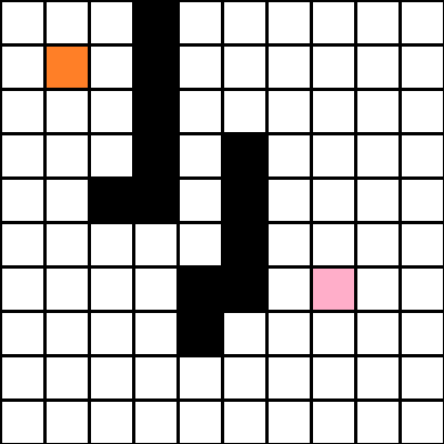
We are given a set of test images, each containing

• A grid of 100 squares of size 40x40 pixels.
• Start marked with a orange square.
• End marked with a pink square.
• Obstacles marked with black squares.

The squares are identified by the coordinate (x,y) where x is the column and y is the row to which the square belongs, as shown in the picture. Assuming a robot moves from Start to End by moving either horizontally or vertically, the objective is to find the shortest path from Start to End. The length of the path is determined by the number of moves the robot makes.

Tools

OpenCV 2.4, an Open-source Computer Vision library is used with Python 2.7. For instructions regarding the installation of OpenCV refer documentation.

Task Analysis

This task more Algorithms based than Image processing. After we convert this image to a graph model, than all that is left is applying a shortest path algorithm to complete the task.

Shortest Path Algorithms

Shortest path algorithms works on Graphs which is a collection of vertices or nodes and edges connecting them. Some of the popular graph representations are adjacency matrix and adjacency list. In adjacency matrix representation a boolean matrix is used, where each entry in matrix represents the relation between ith(row) and jth node(column). A 1 represents the presence of edge and 0 absence. For weighted graphs integer matrix can be used. In adjacency list representation. For more detatils on graph representation read this article.

Dijkstra’s algorithm

Dijkstra’s algorithm works by visiting the vertices in the graph starting with the given starting point. It exaustively examines the unvisited neighbours of current vertex until it reaches the end point. Dijkstra’s algorithm is guaranteed to find the shortest path, where all the edges of graph have a non-negative weight.

Greedy Best First Search algorithm

The Greedy Best First search algorithm on the other hand uses a heuristic i.e. an estimate which determines how far is the goal in selecting the next vertex. So, instead of selecting the vertex closest to starting point, it selects the vertex clsest to the goal, hence greedy. This algorithm computes shortest distance much quicker than Dijkstra’s, but has it’s own pitfalls. First of all Greedy Best First search is not guaranteed to find the shortest path. Also in some cases like in the presence of concave obstacles close to the end point, it can be much slower than Dijkstra’s.

A* Algorithm

A* is one of the most popular choice for pathfinding. It is wide range of applications, especally in Path planning for Robots and Computer games. It combines the heuristic approach of the Best First Search algorithm with the Dijkstra’s algorithm to give a more refined result. It is guaranteed to find the shortest path. It is as fast as Greedy Best first Search but doesn’t suffer from it’s pitfalls.

Note: For in depth analysis of the above algorithms, refer this great article. For animated comparison, please look at this video.

Implementation

• Representing the Image The fist subtask is to convert the image to a matrix representation. For this purpose create a matrix with size corresponding to the rows and column given in problem statement. Traverse this matrix and assign:

  • 0 to traversable blocks
  • 1 to obstacles
  • 2 to start block
  • 3 to end block

1
2
3
4
5
6
7
8
9
10
11
12
13
14
15
grid = np.zeros((rows, columns))
for i in range(rows):
	for j in range(columns):
		# white blocks
		if (np.array_equal(img[20+(i*40), 20+(j*40)], [255, 255, 255])):
			grid[i][j] = 0
		# start -> orange block
		elif (np.array_equal(img[20+(i*40), 20+(j*40)], [39, 127, 255])):
			grid[i][j] = 2
		# end -> pink block
		elif (np.array_equal(img[20+(i*40), 20+(j*40)], [201, 174, 255])):
			grid[i][j] = 3
		# obstacles ->black blocks
		else:
			grid[i][j] = 1

• Representing the Cell We will define some attributes for each cell in the grid.

  • x and y coordinate
  • Parent - The cell from where we reach the current cell.
  • Reachability - If the cell is an obstacle, reachability is false, else true.
  • Cost - The cost of moving to this cell or weight of the node.
  • Heuristic - Measure of distance from goal. Absolute or euclidean distance can be used.
  • Net Cost - Cost + Heuristic

• A* Search Implementing A* requires maintaining two lists i.e. open, closed. The open list contains the cells which are next to be examined and closed list contains cells that have already been examined. To store the information about each cell I have maintained a third list, cells. The data structure used for implementing open list is a min heap which is heapified using Net Cost(cell cost + heuristic). In an abstract description, heap data structure is used to get the cell with lowest net cost around the current cell. Now, we will do a regular Breadth first search on the graph. The major difference would be that instead of a simple queue used in BFS, we will use open list to store the neighboring reachable cells from the current node. Also to keep a track of already examined nodes, move them to closed list. While traversing the graph we will regularly update the parent of the next cell to be visited with current cell which will be used to track the path we have taken. We exit this loop as soon as we reach the node marked as end.

1
2
3
4
5
6
7
8
9
10
11
12
13
14
15
16
17
18
19
20
21
22
23
# pushing the first element in open queue
heapq.heappush(self.open, (self.start.net_cost, self.start))
while(len(self.open)):
	net_cost, cell = heapq.heappop(self.open)
	# adding the checked cell to closed list
	self.closed.add(cell)
	if cell is self.end:
		# store path and path legth
		route_path, route_length = self.display_path()
		route_path.reverse()
		break
	# getting the adjoint cells
	neighbours = self.neighbour(cell)
	for path in neighbours:
		# if cell is not an obstacle and has not been already checked
		if path.reachable and path not in self.closed:
			if (path.net_cost, path) in self.open:
				# selecting the cell with least cost
				if path.cost > cell.cost + 1:
					self.update_cell(path, cell)
			else:
				self.update_cell(path, cell)
				heapq.heappush(self.open, (path.net_cost, path))

Refer my repository for complete code.

Thanks and have a great time implementing your own version of this algorithm!